The Central Limit Theorem is a result in statistics that says that the sum of a bunch of random variables will (under certain loose conditions) approximate the normal distribution.
For simplicity, we will talk here only about the case where the variables being summed up are themselves independent, identically distributed, and with finite variance. Interestingly, the theorem holds in more general situations but with more stipulations that are beyond the scope of this blog post.
I'll first explain the statement of this theorem (mathematically), then explain some of its intuition and lastly give a proof.
Maybe we'll even say something boring about actuarial work too.
Statement (Central Limit Theorem)
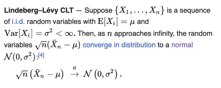
Implications from the formula:
The "sample mean" minus the actual mean converges to N(0, σ^2), which implies the so-called "Law of Large Numbers", which says that if you take the average of a bunch of trials it will get closer and closer to the actual mean of the random variable generating the trials.
The standard deviation of the distribution of how your sample might compare to the actual mean is related to the number of trials by a square root function. Strange! If you take four times as many trials, your bell curve will get half as fat. I've spent a lot of time in the shower trying to internalize this intuition.
There's a lot going on in the statement. Here's a sequential way to think about it:
Imagine you have a random variable for which you know the definitive mean µ and standard deviation σ.
You sample this identical distribution n times and all samples are independent of each other (combined this is what "iid" stands for).
You sum up the results from each sampling and average them.
This "sample mean" itself can be considered a random variable since it is defined in terms of the process above. As a random variable, this sample mean has a distribution that is related to the original distribution by the Central Limit Theorem.
Results:
The distribution of the sample mean is normally distributed around the true mean (no bias)
The distribution of the sample mean has variance related to the variance of the original distribution
The variance of the sample mean decreases by the square root of the number of trials. 100 trials will on average get you 10 times closer to the true mean than one trial would.
The most impressive result of the CLT, though, is probably this:
Nothing except for the variance of the sampled distribution mattered in its eventual convergence to a normal. The sampled distribution could be relatively normal ("average height of people named Bob") or completely skewed ("annual healthcare costs of people named Bob"). Either way, if you sum enough of such samples together, the sample's distribution around the actual mean will smooth out into a symmetric normal distribution.
Intuition
There are two hard parts to intuit about the Central Limit Theorem.
Why is the square root of n the factor by which the distribution converges?
Why is a normal distribution here?
1. Why the square root of n factor?
The square root of n factor roughly describes how quickly convergence happens. The CLT says the width of the bell curve of possible generated sample means gets skinnier by a factor of the square root of the number of samples.
This comes from the fact that variance is additive and standard deviation is the square root of variance. The variance of n independent samples of a distribution will be n times the variance of one sample. The standard deviation will thus be square root of n times the original standard deviation.
Interestingly, the fact that variance is additive is often called the "pythagorean theorem of variance" and can be visualized as such by putting two independent variables on the x and y axes of a graph and visualizing their sum as the coordinate where the two samples converge on the graph. The distance that the coordinate falls from the origin is determined by the pythagorean theorem where the side lengths of the right triangle are determined by the two sampled values.
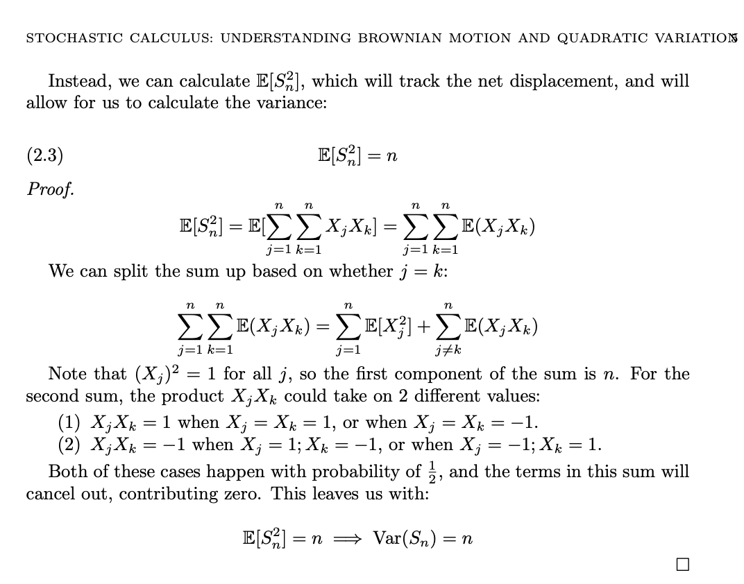
This square root of n term also shows up in Brownian motion, where the expected traveled distance after n unit Brownian motion steps is the square root of n (proof below).
2. Why the normal distribution?
Since most people think of the normal distribution as being defined by its picture or pdf (above right), a lot of people miss that this isn't really a good definition of the normal distribution since it doesn't explain where the normal distribution comes from.
In rigorous statistics courses, the normal distribution is typically defined to be the unique distribution that the sum of independent random variables converge to and then its pdf is determined by computing its moments and normalizing.
If you pay attention to the proof (below) you can see this is essentially what is happening.
So the CLT is a tautology? How lame and useless.
Not at all, the most impressive thing about the CLT is that all random variables that meet its loose conditions wrap up to the same distributions when the sample mean is taken enough times. It is not obvious at all that the distribution of the sample means of almost any random variable all belong to the same normal distribution family.
The "adding" of samples together to produce a converging distribution is indeed the defining property of the normal, which has the unique property that it is the only non-trivial continuous random variable with definite mean and variance for which the sum of two normally distributed random variables is again a normal.
The other "definition" story of the normal is that it is the only non-trivial continuous random variable with definite mean and variance for which the sum of two normally distributed random variables fitting that distribution family also fits the same distribution family.
This makes intuiting why its probability distribution function (pdf) has an exponential with pi in it somewhat easier.
But the story that "you can add these things (normal random variables) together and the sum will be of the same class" is very related indeed to taking sample means, which themselves are just sums of some number of copies of a random variable.
Applications: Inference Statistics
Disclaimer: The CLT is a theorem in so-called "descriptive statistics" that assumes properties of a random variable are known and computes properties of derived random variables.
In reality, we often have the more difficult situation of knowing something about a sample data set, and having to infer properties of the random variable that generated this sample data set.
There are complicated exact solutions to solving for such distributions (including study of the much confused Chi Squared distribution) that help infer properties like the mean and standard deviation of an underlying distribution from just sample data.
In practice though, for large sample sets it is approximately enough to treat the mean and variance of the underlying distribution as equal to the sample mean and sample variance, and apply descriptive statistical methods like CLT calculations without adjustment.
Example application: You are reserving money for an insurance pool (like a captive) and you want to know how the amount of money you have to reserve to handle a two sigma loss changes when the number of iid insured events you are bundling increases from 1000 to 2250 as you write more policies.
The Central Limit Theorem tells us that the standard deviation of our sample mean squeezes by a factor of sqrt(2250/1000) = 1.5 times.
Thus, the odds of a two sigma event with 1000 policies would be equal to the odds of a three sigma event with 2250 policies. So, taking the same amount of proportional reserves per policy, we now can handle more extreme situations and would fail to have enough reserves only 0.3% of the time instead of 2.5% of the time (from basic facts about the normal CDF).
By barely doubling the number of policies pooled together, we are now about 8 times less likely to have insufficient reserves! Incredible.
If instead we still only wanted to reserve against two sigma events, we could reduce our proportional reserves by a factor of 1.5, reducing premiums for insureds.
Proof
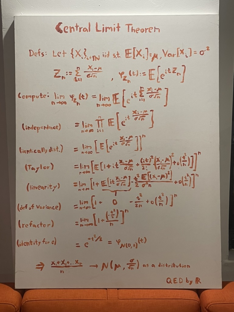
The proof above (and many others) calculates a characteristic function for the distribution of sample means and then shows that this characteristic function is proportional to e^(-t^2/2), which when normalized has the same pdf as the well-known normal distribution.
In the proof, the exp (e^x) term comes from the limit identity of e (below) which is well-known for its "compound interest" story.
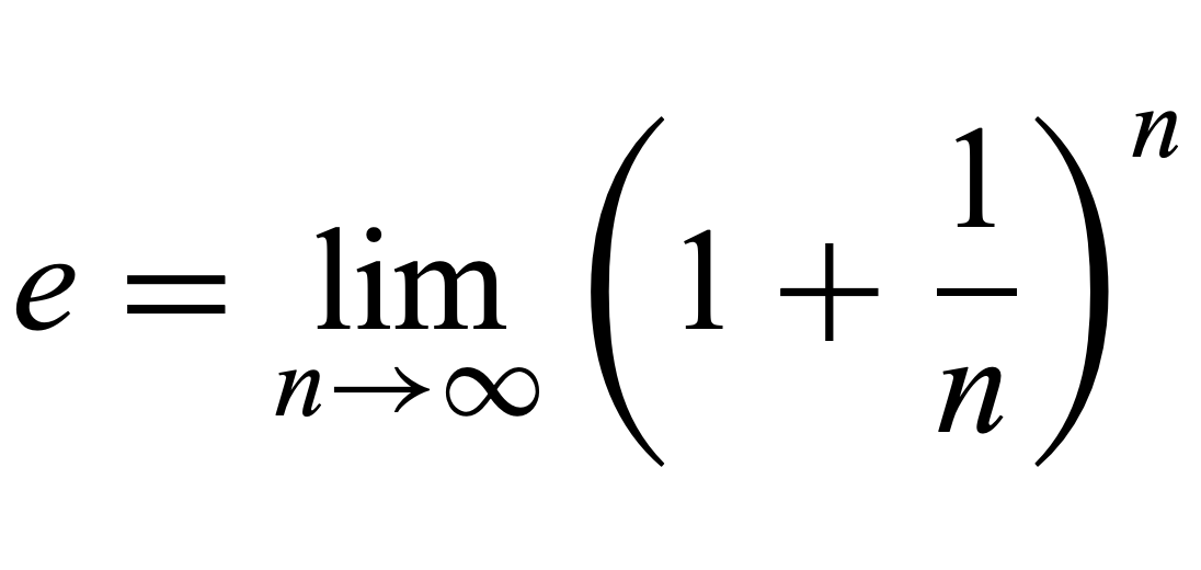
There is again strong intuition here for where e comes from in this pdf. The "infinite sampling" that is computed in the limit of adding the iid random variables together is just like compound interest, an infinitesmal addition to variance being normalized by the number of samples.
The Central Limit Theorem is why insurance works. It shows mathematically why pooling money together from independent risks adds value to each insured by minimizing the variance of their expected losses.
The value gained from this, though, isn't provided by the insurance company itself. Just from math.